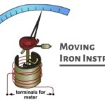
Moving Iron Instrument can measure both AC and DC quantities, which makes it an excellent measurement tool. Although the instrument has the advantage of measuring AC and DC, it also results in some errors. In this article, we examine the errors that can occur in a moving iron instrument.
There are two types of errors in moving iron instruments.
- Errors which occur with both AC and DC
- Errors which occur only with AC only.
Errors with both DC and AC
(i) Hysteresis Error
(ii) Temperature Error.
(iii) Stray Magnetic Fields
1. Hysteresis Error
This error occurs as the value of flux density is different for the same current when ascending and descending. The value of flux density is higher for descending values of current and, therefore, the instrument tends to read higher for descending values of current (and voltage) than for ascending values.
This error can be minimized by making the iron parts small so that they demagnetize themselves quickly. Another method is to work the iron parts at low values of flux density so that the hysteresis effects are small.
Hysteresis may produce a 2 to 3 percent errors in moving iron instruments. With the use of nickel iron alloys with narrow hysteresis loops, the error may be brought down to less than 0.05 per cent.
2. Temperature Error
The effect of temperature changes on moving iron instruments arises chiefly from the temperature coefficient of spring. The error may be 0.02 percent per ℃. In voltmeters, errors are caused due to self-heating of coil and series resistance.
The temperature of the coil may increase by 10 to 20℃ for a power consumption of 1 W. Therefore, the resistance increases (by about 4 to 8%, causing a decrease in current for a given voltage. This produces a decreased deflection. Therefore, the series resistance should be made of a material like Manganin which has a small temperature co-efficient.
The value of series resistance should be very large as compared with the coil resistance in order to minimize errors due to self-heating. In the case of switch board instruments, the series resistance is about 10 times the coil resistance.
3. Stray Magnetic Fields
The errors in moving iron instruments due to stray magnetic fields (fields other than the operating magnetic field) may be appreciable as the operating magnetic field is weak (about 0.006 to 0.0075 Wb/m2 at full scale deflection) and hence can be easily distorted.
Such errors depend upon the direction of the stray magnetic field relative to the field of the instrument. These errors can be minimized by using an iron case or a thin iron shield over the working parts.
Since some types of instruments are not shielded, we should be careful in selecting instruments for places where stray magnetic fields are encountered. If we use an unshielded instrument over a table having metal top or mount such instruments on steel panel, the accuracy may be drastically impaired.
Errors in Moving Iron Instruments with AC only
1. Frequency Errors
Changes in frequency may cause errors due to changes of reactance of the working coil and also due to changes of magnitude of eddy currents set up in the metal parts of instrument.
Reactance of Instrument Coil
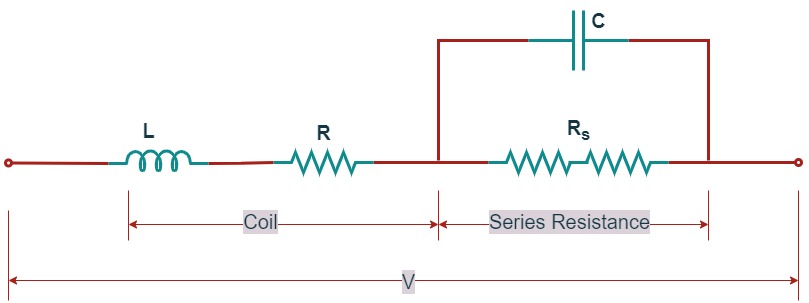
The change of reactance of the instrument coil is important in case of voltmeters where an additional resistance Rs is used in series with the instrument co . Let the resistance and inductance of the instrument coil be R and L.
Then the current I in the instrument coil for a given applied voltage V is given by :
$$
I=\frac{V}{\sqrt{\left(R+R_s\right)^2+\omega^2 L^2}}
$$
The deflection of the moving-iron voltmeter depends upon the current through the coil. Therefore, the deflection for a given voltage will be less at high frequencies than at low frequencies. To some extent, compensation to this type of error is possible by connecting a capacitor $C$ across the series resistance Rs as shown in figure.
The idea of shunting the series resistor is to make the circuit behave like a pure resistance so that the frequency changes have no effect on the readings of the instrument. Thus the compensated instrument will have a power factor nearly equal to unity. As the resistance of the meter, R, is considerably smaller than the series multiplier resistance Rs, it can be assumed that it is sufficient to ensure that the magnitude Z of the impedance of the circuit. formed by L, Rs, and C has a value Rs under AC conditions.
Now $\quad \mathrm{Z}=j \omega L+\frac{R_s}{1+j \omega C R_s}=j \omega L+\frac{R_1-j \omega C R^2}{1+\omega^2 C^2R_s^2}$
Since $\omega C R_s \ll 1$, we can write $Z=j \omega L+\left(R_s-j \omega C R_s{ }^2\right)\left(1-\omega^2 C^2 R_s^2\right)$
$=j \omega L+R_s-j \omega C R_1{ }^2-\omega^2 C^2 R_s{ }^3+j \omega^2 C^2 R_s^4$
$=R_s-\omega^2 C^2 R_s{ }^3+\mathrm{j}\left[\omega L-\omega C R_s{ }^2\left(1-\omega^2 C^2 R_8{ }^2\right)\right]$
$\simeq R_s-\omega^2 C_3^2 R_s{ }^3+j\left[\omega L+\omega C R_s{ }^2\right]$
$=R_s\left(1-\omega^2 C^2 R_s{ }^2\right)+j\left[\omega L-\omega C R_s{ }^2\right]$
Magnitude of $Z^2=R_s{ }^2\left(1+\omega^2 C^2 R_s{ }^2\right)^2+\omega^2\left(L-C R_3{ }^2\right)^2j$
This must equal $R_s{ }^2$ in order that the a c. calibration at all frequencies and d.c. calibration is the same.
$\therefore R_s{ }^2=R_s{ }^2\left(1-\omega^2 C^2 R_s{ }^2\right)^2+\omega^2\left(L-C R_s{ }^2\right)^2$
$=R_s{ }^2\left(1+\omega^2 C^4 R_s^4-2 \omega^2 C^2 R_s{ }^2\right)+\omega^2\left(L-C R_s{ }^2\right)^2$
$=R_s{ }^2(\left(-2 \omega^2 C^2 R_s{ }^2+\omega^4 C^4 R_s^4\right)+\omega^2\left(L-C R_s\right)^2$
$=R_s{ }^2\left(1-2 \omega^2 C^2 R_s{ }^2\right)+\omega^2\left(L-C R_s{ }^2\right)^2\ as\ \omega^4 C^4 R_s{ }^2<1$
$=R_s^2-2 \omega^2 C^2 R_s^4+\omega^2 L^2+\omega^2 C^2 R_s^4-2 \omega^2 L C R_s^2$
Thus $0=\omega^2 L^2-\omega^2 C^2 R_s^4-2 \omega^2 L C R_s^2$.
$$L^2-2 L C R_s{ }^2-C^2 R_s^4=0$$
$$L=\frac{2 C R_s{ }^2+\sqrt{4 C^2 R_s^4+4 C^2 R_s^4}}{2} =2.41 C R_s{ }^2$$ $$C=\frac{1}{2 \cdot 41} \frac{L}{R_s^2}=0.41 \frac{L}{R_s{ }^2}$$
In practice it is usual to consider the variation of Z within certain limits for the DC value R+Rs. Figure shows the frequency error with and without compensation.
It may be observed that for an uncompensated instrument the error goes beyond permissible limits for frequencies above $\omega_1$. With compensation the frequency range is extended from $\omega_1$ to $\omega_2$ and in fact the instrument current at a frequency $\omega_3$ is the same as with DC.
2. Eddy Currents
These errors are caused by eddy currents induced in the iron parts of the instruments. Let the mutual inductance between the instrument coil and the iron parts be $M$. The induced voltage $E_b(=\omega M I)$ due to current $I$ in the instrument coil lags the current by $90^{\circ}$. As a result of this induced voltage an eddy current $I_e$ flows and its magnitude is
$$
I_\theta=\frac{\omega M I}{\sqrt{\bar{R}\theta^2+\omega^2 L\theta^2}}
$$
where $R_0$ and $L_0$ are respectively the resistance and inductance of this eddy current path. Io lags $E_s$ by an angle $\theta_0=\tan ^{-1} \frac{\omega L_0}{R_0}$
A component of this current $I_e^{\prime}-I_\theta \cos \left(90-\theta_\theta\right)=I_0 \cdot \operatorname{lin} \theta_e$ opposes the instrument current I and sets up on opposing field thus reducing the torque on the moving system. From tho phasor diagram sketched in Fig. $8.37$, it is seen
$$
I_{l^{\prime}}^{\prime}=I_{\theta_0^{\prime}}^{\prime} \sin \theta_\theta=\frac{\omega M I}{\sqrt{R_0^6+\omega^2 L}} \cdot \frac{\omega L_t}{\sqrt{R_{\varphi^8}{ }^2+\omega^8 L_0^2}}
$$
$$
=\frac{\omega^2 M L_\theta I}{R_0^2+\omega^2 L_0^2}
$$
$\therefore \quad I^{\prime} \frac{\omega^2 M L_e I}{R \theta^2}$ when $R e \omega L_i$, t.e, when $\omega$ is small.
$I_{\circ} \approx \frac{M I}{L_{\mathrm{t}}}$ when $\omega L_0>R_0$ le. $_{\text {., }}$ when $\omega$ is large.
Thus at low frequencies the eddy current error increases with square of the frequency while at high frequencies the error is practically constant. For these reasons moving iron instruments are unsuitable for frequencies above 100 Hz.
In order to extend the frequency range of the Instrument, another coil, coupled with the coil of the instrument and loaded by an AC network, is used. The frequency errors in moving iron instruments due to eddy currents can be kept less than 0.1 % up to a frequency range of 1000 Hz.
Conclusion
| Type of Error | Cause | Minimization Method |
|---|---|---|
| Errors in Both AC and DC | ||
| 1. Hysteresis Error | Different flux density for ascending and descending currents | Use small iron parts, operate at low flux density, use nickel iron alloys |
| 2. Temperature Error | Temperature coefficient of spring and self-heating of coil | Use materials with small temperature coefficients (e.g., Manganin), increase series resistance |
| 3. Stray Magnetic Fields | Influence of external magnetic fields | Use iron case or thin iron shield, avoid metal tables or steel panels |
| Errors in AC Only | ||
| 1. Frequency Errors | Changes in reactance of the working coil and eddy currents | Connect a capacitor across the series resistance to make the circuit behave like a pure resistance |
| 2. Eddy Currents | Induced eddy currents in iron parts, opposing instrument current | Use an additional coil coupled with the instrument coil and loaded by an AC network |
Comments are closed.