Signals are a fundamental concept in the field of engineering and play a critical role in communication systems, control systems, and other areas. Signals can be broadly categorized into two types based on their time domain – continuous-time signals and discrete-time signals.
A continuous-time signal is a signal that varies smoothly over an infinite range of time, whereas a discrete-time signal is a signal that changes only at specific instances in time.
Understanding the difference between these two types of signals and their properties is crucial in the design and analysis of various engineering systems. In this context, this article aims to provide an overview of continuous-time signals and discrete-time signals, their properties, and their applications.
Continuous Time Signal
Definition
A signal that varies smoothly and continuously over time is referred to as a continuous-time signal. These signals represent a quantity of interest that is influenced by an independent variable, usually considered as time.
Voltage readings at a node in an electrical circuit and the temperature fluctuations at a particular location in a room are two examples of continuous-time signals that depend on time as the independent variable.
A more precise, mathematical definition of continuous time signal is:
A continuous-time signal is a function x(t) of the real variable t defined for −∞ < t < ∞ .
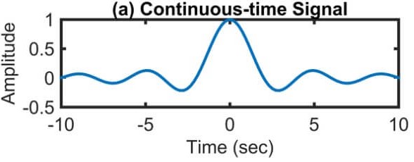
Continuous time signal representation as shown in the sketch below.
On planet earth, physical quantities take on real numerical values, though it turns out that sometimes it is mathematically convenient to consider complex-valued functions of t. However, the default is real-valued x(t), and indeed the type of sketch exhibited above is valid only for real-valued signals. A sketch of a complex-valued signal x(t) requires an additional dimension or multiple sketches, for example, a sketch of the real part, Re{x(t)}, versus t and a sketch of the imaginary part, Im{x(t)}, versus t .
Properties of continuous-time signals
- A continuous-time signal is not necessarily a continuous function, in the sense of calculus. Discontinuities (jumps) in a signal are indicated by a vertical line, as drawn above.
- The default domain of definition is always the whole real line – a convenient abstraction that ignores various big-bang theories. We use ellipses as shown above to indicate that the signal “continues in a similar fashion,” with the meaning presumably clear from context. If a signal is of interest only over a particular interval in the real line, then we usually define it to be zero outside of this interval so that the domain of definition remains the whole real line. Other conventions are possible, of course. In some cases a signal defined on a finite interval is extended to the whole real line by endlessly repeating the signal (in both directions).
- The independent variable need not be time, it could be distance, for example. But for simplicity we will always consider it to be time.
- An important subclass of signals is the class of unilateral or right-sided signals that are zero for negative arguments. These are used to represent situations where there is a definite starting time, usually designated t = 0 for convenience.
Example of Continuous Time Signal
A continuous signal is specified at every value of its independent variable. For example, the temperature of a room is a continuous signal.
One cycle of the continuous complex exponential signal, $x(t)=e^{j\left(\frac{2 \pi}{16} t+\frac{\pi}{3}\right)}$ , is shown in figure below.
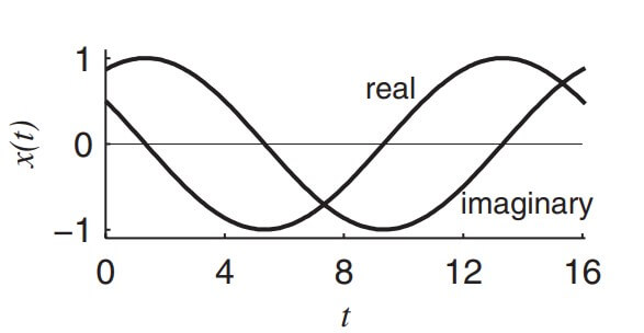
We denote a continuous signal, using the independent variable t, as x(t). We call this representation the time-domain representation, although the independent variable is not time for some signals. Using Euler’s identity, the signal can be expressed, in terms of cosine and sine signals, as
$$
x(t)=e^{j\left(\frac{2 \pi}{16} t+\frac{\pi}{3}\right)}=\cos \left(\frac{2 \pi}{16} t+\frac{\pi}{3}\right)+j \sin \left(\frac{2 \pi}{16} t+\frac{\pi}{3}\right)
$$
Thereal part ofx(t) is thereal sinusoid $\cos \left(\frac{2 \pi}{16} t+\pi / 3\right)$ and the imaginary part is thereal sinusoid $\sin \left(\frac{2 \pi}{16} t+\pi / 3\right)$, as any complex signal is an ordered pair of real signals. While practical signals are real-valued with arbitrary amplitude profile, the mathematically well-defined complex exponential is predominantly used in signal and system analysis.
Discrete Time Signal
A discrete-time signal is a sequence of values of interest, where the integer index can be thought of as a time index, and the values in the sequence represent some physical quantity of interest.
Because many discrete-time signals arise as equally-spaced samples of a continuous-time signal, it is often more convenient to think of the index as the “sample number.” Examples are the closing Dow-Jones stock average each day and the room temperature at 6 pm each day. In these cases, the sample number would be day 0, day 1, day 2, and so on.
Definition
We use the following mathematical definition.
A discrete-time signal is a sequence x[n] defined for all integers −∞ < n < ∞ .
We display x[n] graphically as a string of lollypops of appropriate height.
A discrete-time signal x[n] may represent a phenomenon for which the independent variable is inherently discrete. For instance, the daily closing stock market average is by its nature a signal that evolves at discrete points in time (that is, at the close of each day). On the other hand a discrete-time signal x[n] may be obtained by sampling a continuous-time signal x(t) such as
x(t0),x(t1), …,x(tn),…
or in a shorter form as
x[0],x[1], …,x[n], …
or x0,x1,…,xn,…
where we understand that
xn = x[n] = x(tn)
and xn‘s are called samples and the time interval between them is called the sampling interval.
When the sampling intervals are equal (uniform sampling), then
xn = x[n] = x(nTs)
where the constant Ts is the sampling interval
Representation of Discrete Time Signals
A discrete-time signal x[n] can be represented in two ways:
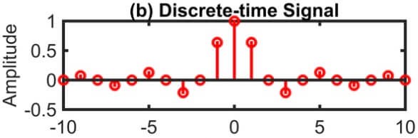
1. We can specify a rule for calculating the nth value of the sequence. For example,
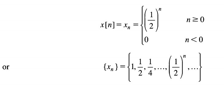
2. We can also explicitly list the values of the sequence.
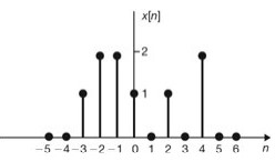
For example, the sequence shown in figure above can be written as
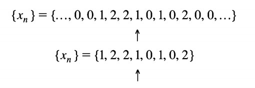
We use the arrow to denote the n = 0 term. We shall use the convention that if no arrow is indicated, then the first term corresponds to n= 0 and all the values of the sequence are zero for n < 0.
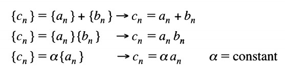
The sum and product of two sequences are defined as follows:
Example of Discrete Time Signal
A discrete signal is specified only at discrete values of its independent variable.
For example, a signal x(t) is represented only at t = nTs as x(nTs), where Ts is the sampling interval and n is an integer.
The discrete signal is usually denoted as x[n], suppressing Ts in the argument of x(nTs). The important advantage of discrete signals is that they can be stored and processed efficiently using digital devices and fast numerical algorithms.
As most practical signals are continuous signals, the discrete signal is often obtained by sampling the continuous signal. However, signals such as yearly population of a country and monthly sales of a company are inherently discrete signals.
Whether a discrete signal arises inherently or by sampling, it is represented as a sequence of numbers {x(n), −∞ < n < ∞}, where the independent variable n is an integer. Although x(n) represents a single sample, it is also used to denote the sequence instead of {x(n)}.
One cycle of the discrete complex exponential signal, $x(n)=e^{j\left(\frac{2 \pi}{16} n+\frac{\pi}{3}\right)}$, is shown in figure below.
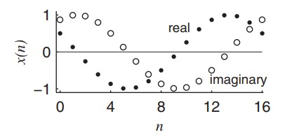
This signal is obtained by sampling the signal (replacing t by nTs) in continuous time signal with Ts = 1 s. We assume that the sampling interval, Ts, is a constant. In sampling a signal, the sampling interval, which depends on the frequency content of the signal, is an important parameter.
The sampling interval is required again to convert the discrete signal back to its corresponding continuous form. However, when the signal is in discrete form, most of the processing is independent of the sampling interval. For example, summing of a set of samples of a signal is independent of the sampling interval.
Differences between Continuous Time and Discrete Time Signal
The differences between CTS and DTS are tabulated below
| Continuous Time Signal | Discrete Time Signal |
| The continuous-time signal is an analog representation of a natural signal. | The discrete-time signal is a digital representation of a continuous-time signal. |
| The continuous-time signal can be converted into discrete-time signal by the Euler’s method. | The discrete ~time signal can be converted into continuous-time signal by the methods of zero-order hold or first-order hold. |
| The conversion of continuous to discrete-time signal is comparatively easy than the conversion of discrete to continuous-time signals. | The conversion of discrete to continuous- time signals is very complicated and it is done through a sample and hold process. |
| It is defined over a finite or infinite domain of sequence. | It is defined over a finite domain of sequence. |
| The value of the signal can be obtained at any arbitrary point of time. | The value of the signal can be obtained only at sampling instants of time. |
| The continuous-time signals are not used for the processing of digital signals. | The discrete-time signals are used for the processing of digital signals. |
| The continuous-time variable is denoted by a letter t. | The discrete-time variable is denoted by a letter n. |
| The independent variable encloses in the parenthesis (.). | The independent variable encloses in the bracket [.]. |
Digital Signal
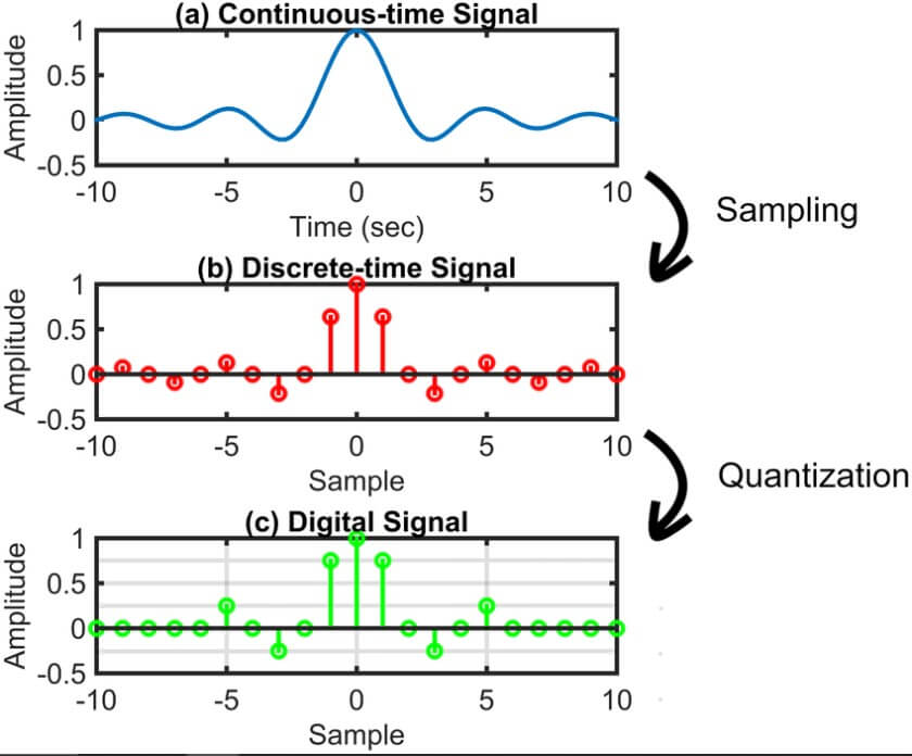
A digital signal can be either discrete-time or continuous-time. Although not all digital signals are discrete-time, they all have a discrete value at each sampling point. These signals are commonly used to represent data as a sequence of discrete values.
When the sample values of a discrete signal are quantized, it becomes a digital signal. That is, both the dependent and independent variables of a digital signal are in discrete form.
This form is actually used to process signals using digital devices, such as a digital computer.
When a signal is transformed into a digital signal, it is converted into binary bits. These bits consist of either a 0 or a 1, with 1 indicating a positive value of the digital signal and 0 representing no value or a zero value. Digital signals are typically represented by a square wave, and the transition from one bit value to another occurs instantaneously. At any given moment, a digital signal can take on one of a finite number of values.
Advantages of Digital Signals
Digital signals have several advantages over analog signals. Firstly, digital signals are less affected by noise, distortion, and interference, which leads to higher signal quality and reliability.
Secondly, digital data can be compressed more easily than analog data, making transmission more efficient. This is because digital signals only need to transmit the ones and zeros that represent the signal, whereas analog signals transmit a continuous waveform.
Thirdly, digital signals offer better security because they can be encrypted and decrypted easily. This makes them ideal for transmitting sensitive information such as financial data, medical records, and classified information.
Fourthly, digital signals can be easily upgraded by simply updating the software or hardware that processes them. This makes it easier to add new features and improve performance.
Fifthly, digital signals are easier to design than analog signals because they can be programmed using software tools. This makes it easier to create complex signal processing algorithms and filters.
Sixthly, digital signals can improve error performance and signal quality by using error correction and detection algorithms. This results in a more accurate and reliable transmission of data.
Seventhly, digital signals are cost-effective compared to analog signals for the transmission of data. This is because digital signals require less expensive equipment and can transmit data over longer distances with less signal degradation.
Lastly, digital signals can be easily stored using less memory and in a shorter duration compared to analog signals. This makes it easier to store and retrieve large amounts of data efficiently.
Differences between Discrete and Digital Signals
The differences between discrete and digital signals are tabulated below.
| Discrete Time Signal | Digital Signal |
| The discrete-time signal is a digital representation of a continuous-time signal. | The digital signal is a form of discrete-time signal. |
| The discrete -time signal can be obtained from the continuous-time signal by the Euler’s method. | The digital signal can be obtained by the process of sampling, quantization, and encoding of the discrete-time signal. |
| The discrete-time signal is a signal that has discrete in time and discrete in amplitude. | The digital signal is a signal that has discrete in amplitude and continuous in time. |
| The value of the signal can be obtained only at sampling instants of time. | The amplitude of the digital signal is either 1 or 0. That is, either OFF or ON. |
| The signals are sampled but not necessary to quantized in the discrete-time signals. | The signals are sampled and quantized in the digital signals. |
| All the discrete-time signals are digital signals. | All the digital signals are not discrete- time signals. |